If you’ve been following the LOD series on PetroChromatics, you’ll know that we’ve already covered the simple S/N-based approaches. In this post, we’ll take things one step deeper with the GC LOD standard deviation method — a more statistically robust approach that’s commonly accepted by academic institutions and scientific bodies. Although it takes a bit more effort, the clarity and confidence it provides are absolutely worth it.
Why the GC LOD Standard Deviation Method Matters
Unlike fast S/N shortcuts, the GC LOD standard deviation approach uses actual variability from multiple blank runs. Because of that, it captures the true spread of your noise distribution. This method is rooted in classic statistics and aligns closely with ICH, EPA, and ASTM thinking.
Before we get into formulas, let’s revisit something familiar: the normal distribution curve.
Understanding the Gaussian Basis of the GC LOD Standard Deviation Method
Here is the type of plot we’re working with — a normal distribution with ±3 standard deviations from the mean:

Statistically, 99.73% of all values fall between −3SD and +3SD. That means only 0.27% of the values fall outside this range. If a value lies outside the ±3SD band, it probably does not belong to the same population.
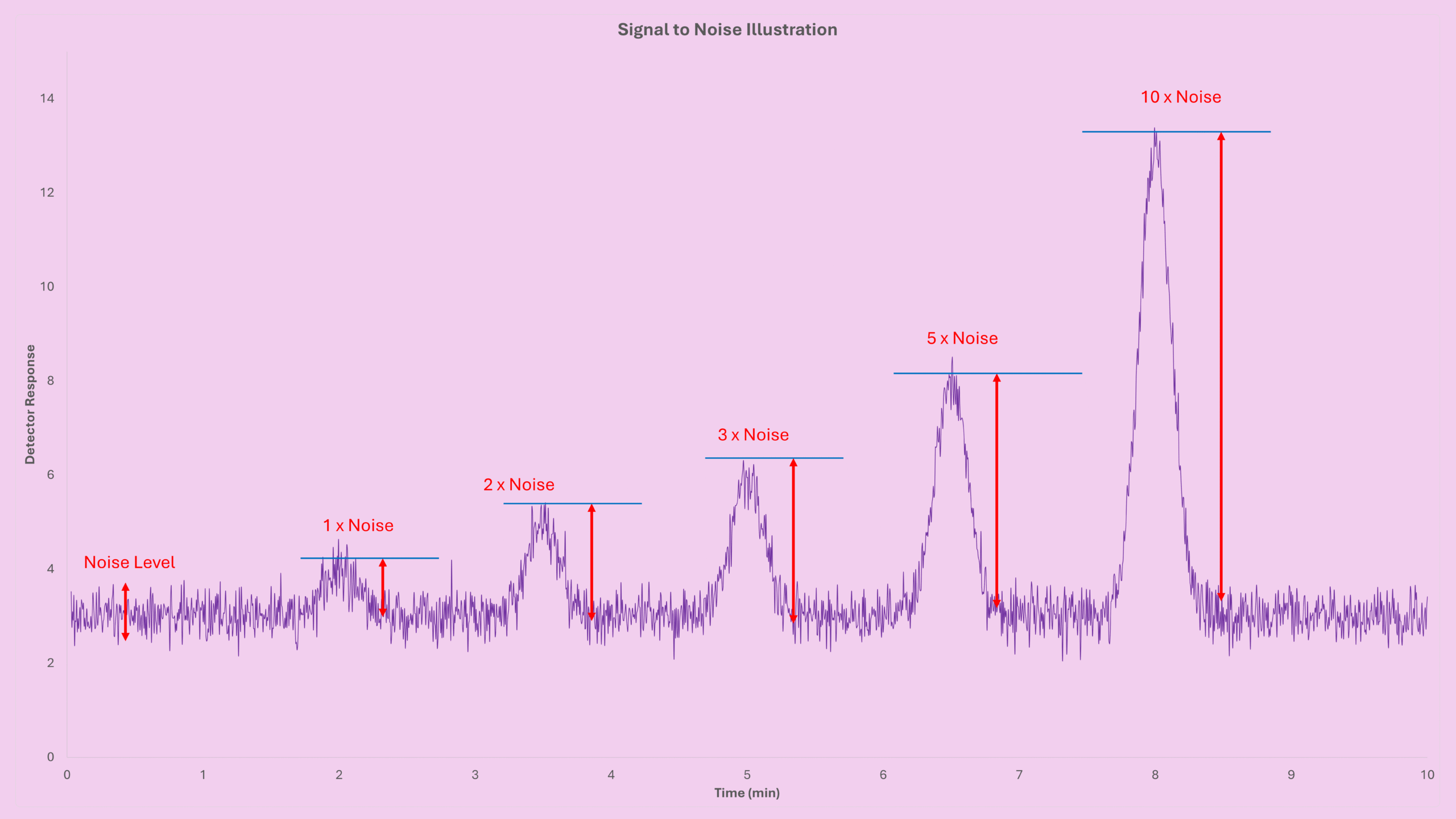
Now imagine that the “population” is simply your noise. If a new measurement falls outside the noise distribution, we can confidently say it is distinguishable from noise.
This leads to an important conclusion:
A signal is distinguishable from noise when:
Value > Mean + 3 × SD
This is the heart of the GC LOD standard deviation method.
Applying the GC LOD Standard Deviation Method to Real GC Data
Let’s say you run 20 blank samples, and each blank shows a tiny peak labeled “methanol.” You record the peak areas of these 20 methanol peaks and plot them:

In your test sample, you detect another methanol peak. So the question becomes:
Is this methanol peak truly from the sample, or is it indistinguishable from noise?
We simply compare:
If TestPeakArea > MeanBlank + 3 × SDBlank
→ It is a true measurable signal.
Else
→ It is not distinguishable from noise.
This gives us the formula:
LOD = MeanBlank + 3 × StandardDeviationBlank
Choosing the Number of Blank Runs (Why 8 Is the Practical Minimum)
Although 20 runs are ideal, realistically most labs cannot dedicate that much instrument time. Running too few blanks, however, gives unstable standard deviation estimates.
The practical compromise?
👉 At least 8 blank runs.
This gives a reasonable estimation of mean and SD while keeping the workload manageable.
Excel makes this step easy:
Mean = AVERAGE(A1:A8)
SD   = STDEV.P(A1:A8)
Why STDEV.P?
Because we treat blank noise as a “population,” not a sample. Most regulatory and scientific bodies also default to population SD for noise-based LOD.
Converting Area-Based LOD to Concentration-Based LOD
So far, everything is based on area. To convert LOD into concentration, we use the slope and intercept of your calibration curve:
Calib: Area = Slope × Concentration + Intercept
Rearranging gives:
Concentration = (Area − Intercept) / Slope
Therefore:
MeanConcentration = (MeanArea − Intercept) / Slope
SDConcentration   = SDarea / Slope
Then the final LOD (in concentration units) is:
LOD = MeanConcentration + 3 × SDConcentration
And, as usual:
LOQ = 3.3 × LOD
Key Takeaways
- The GC LOD standard deviation approach is statistically strong and widely accepted.
- LOD is defined as:
LOD = MeanBlank + 3 × SDBlank - Use at least 8 blank runs for stability.
- Use STDEV.P, not STDEV.S.
- Conversion to concentration uses your calibration slope and intercept.
- LOQ remains 3.3 × LOD.
Before You Go
If this guide helped clarify the LOD by standard deviation method, you’ll probably enjoy the rest of the Detection Limit (LOD/LOQ) series and the GC Free Calculators on my site. Feel free to share the post with your team — it might save someone hours of confusion the next time they struggle with LOD determination.