If you’ve been following the LOD series, this post will take you into the most widely accepted approach of all: the GC LOD residual SD method. Unlike earlier topics where everything revolved around blank noise or blank variability, this approach captures all sources of variation — from sample prep, injection, detector drift, to calibration scatter. Because it reflects the real-world variability of your complete method, it is considered the most scientifically rigorous way to estimate LOD.
Let’s break it down in a friendly, digestible way. And as always, a ready-to-use calculator is available at the top of this post so you don’t have to build one yourself.
Why the GC LOD Residual SD Method Is So Powerful
The GC LOD residual SD approach pulls noise information not from blanks, but from the scatter of your calibration curve. This includes:
- instrument drift
- detector response fluctuations
- injection variability
- integration inconsistency
- and even minor non-linearity
Because all these factors influence uncertainty, this method treats them as contributors to noise — making your LOD estimate more representative of the real world.
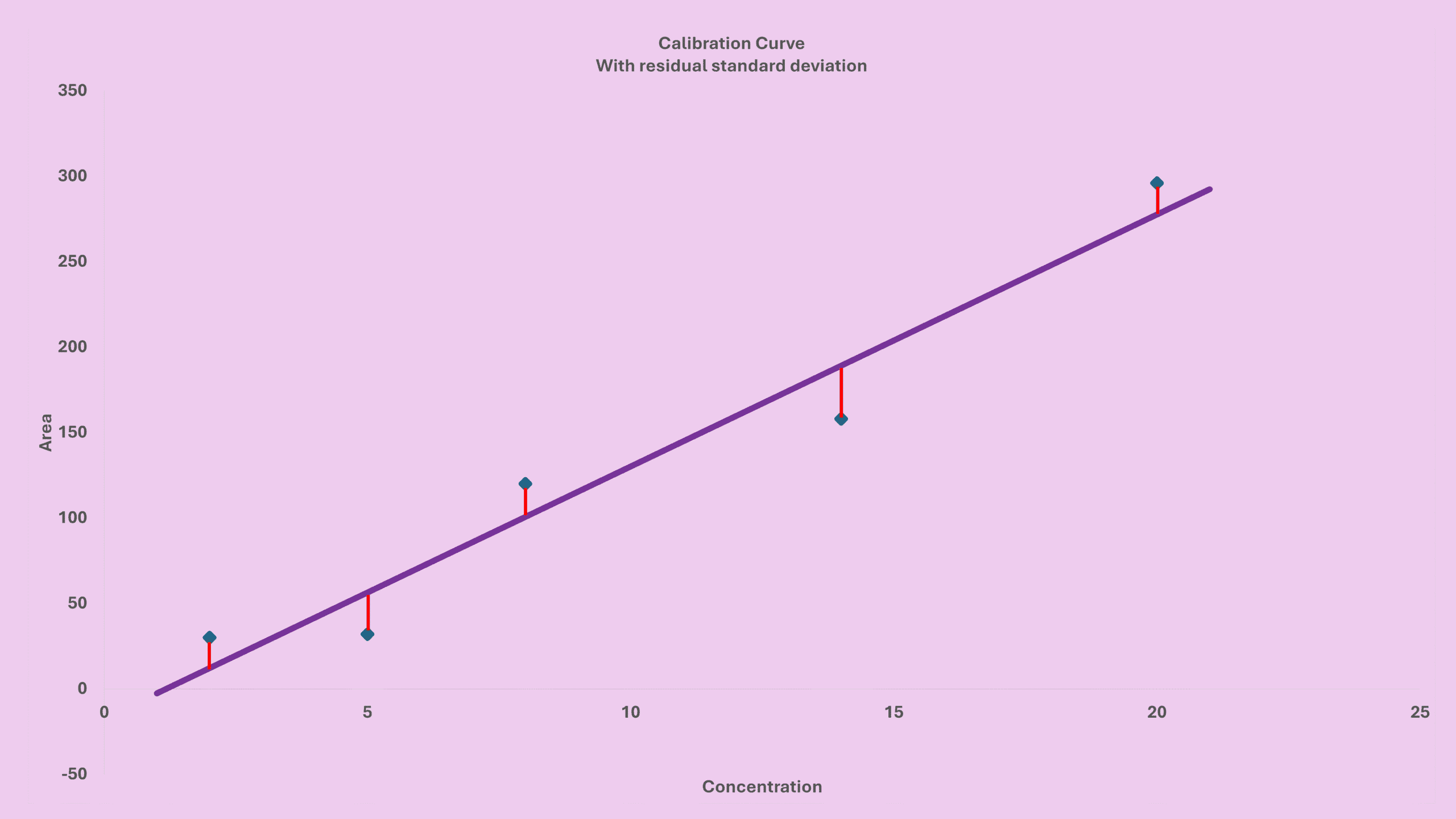
To visualize this, imagine a 5-point calibration curve where each point doesn’t sit perfectly on the regression line. The vertical red lines represent how far each true measured area differs from the area predicted by the curve.

These differences are called residuals, and they form the foundation of this LOD approach.
Calculate Residual Standard Deviation for GC LOD Residual SD Approach
Residuals can be positive or negative, so they must be squared before summing. The formula for residual standard deviation is:
Residual SD = √( Σ(RealAreaᵢ − CalculatedAreaᵢ)² / (n − 2) )
Where:
- n = number of calibration levels
- subtracting 2 accounts for slope and intercept estimation
This value represents the overall noise of your system.
In a perfect world where every calibration point lies exactly on the regression line, residual SD would be zero. But in real GC labs? That never happens — and that’s why this method works so well.
LOD Formula for the GC LOD Residual SD Method
Once residual SD is computed, LOD is derived using this simple and powerful formula:
LOD = (3.3 × Residual SD) / Slope
Why 3.3 instead of 3?
It’s largely convention. Some scientific bodies use 3; others use 3.3. Both are acceptable, but the GC LOD residual SD method traditionally uses 3.3.
And for LOQ:
LOQ = 3 × LOD
Step-By-Step Example Using a 5-Point Calibration
Let’s walk through the full calculation using this dataset:
| Level | Concentration (ppm) | Area |
|---|---|---|
| 1 | 2 | 35 |
| 2 | 5 | 173 |
| 3 | 8 | 345 |
| 4 | 14 | 702 |
| 5 | 20 | 1750 |
1. Compute slope & intercept
In Excel:
Slope     = SLOPE(B1:B5, A1:A5)
Intercept = INTERCEPT(B1:B5, A1:A5)
2. Compute theoretical (predicted) areas
Use:
=A1*$Slope + $Intercept
Drag down for all rows.
3. Compute squared residuals
Use:
=SUMXMY2(B1:B5, C1:C5)
Where column C contains theoretical areas.
4. Compute residual SD
Residual SD = SQRT( SUMXMY2 / (n − 2) )
For this example:
Residual SD = 2.897347261
5. Compute LOD
LOD = (3.3 × 2.897347261) / 35.04266874
LOD = 0.27 ppm
6. Compute LOQ
LOQ = 3 × LOD
LOQ = 0.82 ppm
All these formulas are already built into the calculator at the top of this post.
Key Takeaways
- The GC LOD residual SD method captures all sources of variability.
- It is the most accepted LOD estimation approach among scientific bodies.
- Residual SD comes from the scatter of your calibration curve.
- Minimum 4 calibration levels is recommended (ideally 5+).
- Final LOD formula:
LOD = (3.3 × Residual SD) / Slope
Try the GC LOD Residual SD Instant Calculator
A calculator that implements the approach discussed in this blog post can be found at GC LOD Calculator – Residual Standard Deviation. Just enter:
- Concentrations of a target compound used to build its calibration curve
- Peak areas of a target compound used to build its calibration curve
The result updates automatically — perfect for method development, detector comparison, and troubleshooting.
Before You Go
If this explanation of the GC LOD residual SD method helped clarify how real-world variability contributes to LOD, feel free to explore the rest of the LOD series and try the calculators. A deeper understanding of these tools makes GC method development not just easier — but genuinely satisfying.
To explore earlier posts in this series:


