Understanding Gaussian Distribution Chromatography in Practical GC Work

In this post, I will touch base on something quite confusing as the way it sounds: Gaussian distribution chromatography or normal distribution. I’m not trying to put in all formula and academic stuff, but instead focus on how to apply this concepts in our daily work, especially chromatography.

Even though it’s a confusing concept, most of us have seen or even applied it. For example, the peak you get from a chromatogram. When it looks sharp and symmetric, we often call it a Gaussian distribution peak, or simply a perfect peak.

So in this post, I will touch on two separate sub-concepts that become much clearer once you understand this concept:

• Gaussian distribution in random data, such as noise
• Gaussian distribution for chromatography peak

---

Gaussian Distribution Chromatography Formula Basics

Before diving in, let’s just get to the formula of Gaussian distribution chromatography:

\[ f(x)=\frac{1}{\sigma\sqrt{2\pi}} e^{-\frac{(x-\mu)^2}{2\sigma^2}} \]

Look scary? Luckily, we are not mathematicians, so we do not need to deal with the formula as a whole. Instead, we only extract what we need from the formula for practical use.

What each term means

• x represents the value we need to evaluate, for example noise value
• μ represents the mean value of those x values
• So x − μ tells us how far the current x value is from the center
• Squaring it removes the sign, so no need to worry about left or right
• σ represents standard deviation
• The front term is a normalization factor

---

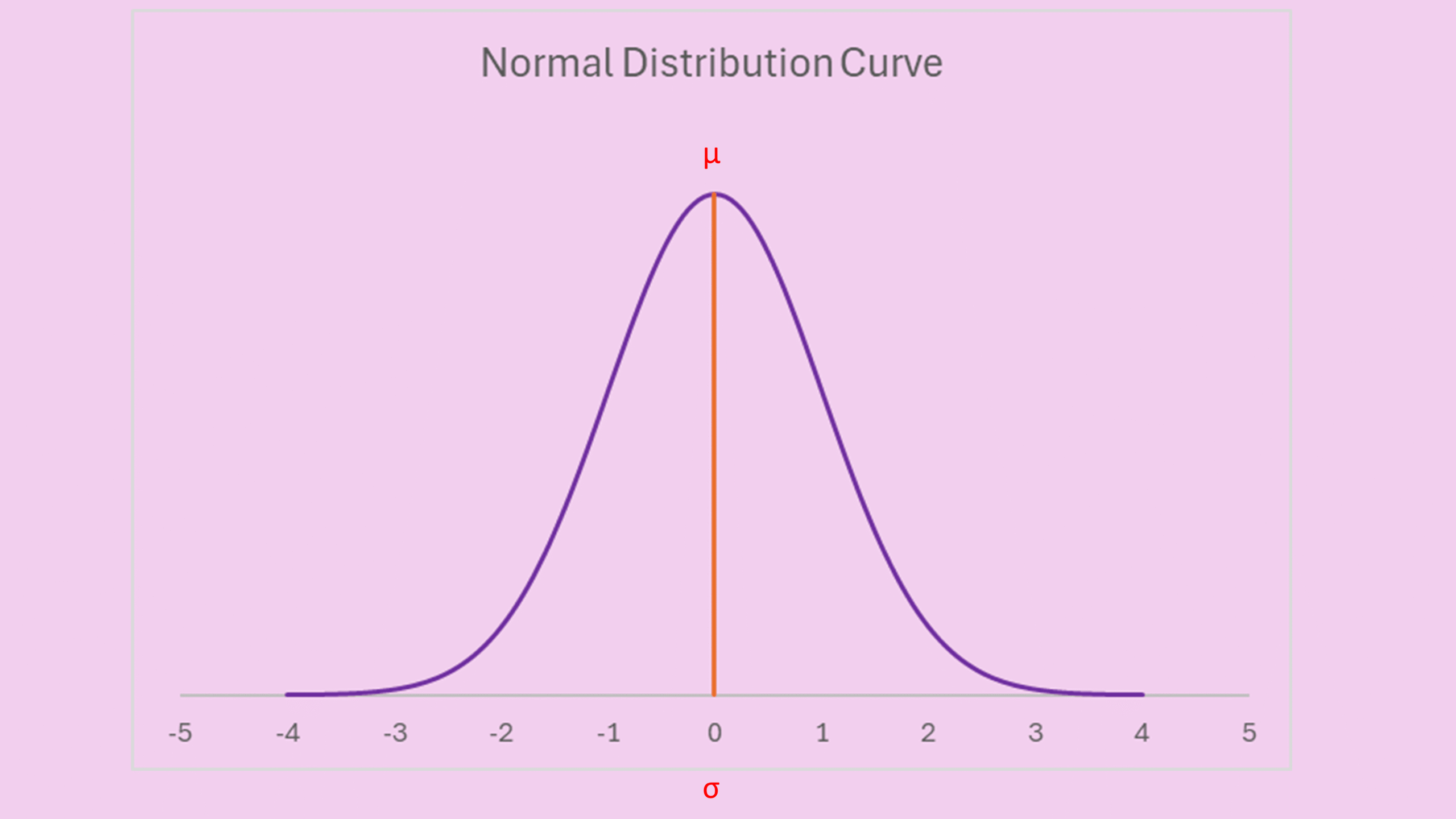
Understanding σ in Gaussian Distribution Chromatography

In summary:

• μ is at the center of the curve
• σ represents the width of the curve

However, σ is not the width itself. Instead, it defines how the curve spreads.

The normalization factor ensures the total area under the curve stays constant. As σ increases, the peak becomes broader. Conversely, when σ decreases, the peak becomes sharper.

---

Area Under the Curve in Gaussian Distribution Chromatography

When it comes to area under the curve, we normally think about integration. However, the Gaussian distribution integral cannot be solved manually. Fortunately, Excel handles this easily.

Using Excel:

=NORM.DIST(-4,0,1,TRUE)

This gives a very small value (~0.00317%), meaning very little contribution exists beyond -4σ. Since the curve is symmetric, the same applies to +4σ.

So the area between -4σ and +4σ is approximately:

=100% - 0.000317% - 0.000317%
=99.99366%

In summary:

• 99.99366% at 4σ
• 99.73002% at 3σ
• 95.44997% at 2σ
• 68.26895% at 1σ

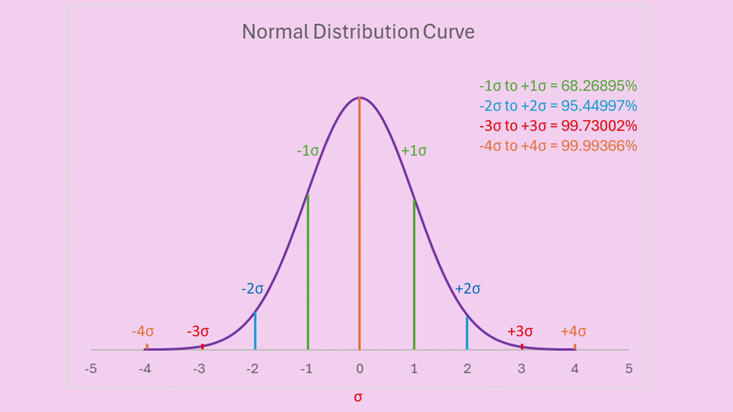
Because 3σ and 4σ already cover more than 99% of the area, they are often used as practical boundaries in representing the whole area.

• 4σ each side → total width = 8σ
• 3σ each side → total width = 6σ

---

Gaussian Distribution Chromatography in Random Data (Noise)

Now let’s move into real applications of this concept.

First, consider random data such as noise. Many real-life examples follow Gaussian distribution. For instance, height distribution in a population or baseline noise in chromatography.

Most values cluster around the mean, while only a few appear as outliers.

If you repeat measurements multiple times, most results will stay near the mean, and only a few deviate. Therefore, to observe this behavior clearly, you typically need at least 20 data points.

---

Connection to LOD

In my previous post on LOD, I discussed this concept using Gaussian distribution chromatography.

When performing blank runs:

• Responses follow normal distribution
• Most values stay within ±3σ

So if a signal exceeds 3σ, there is a 99.73% chance that the signal is real, not noise.

👉 GC LOD Standard Deviation: A Clear Guide to the 3×SD Detection Limit Method

---

Gaussian Distribution Chromatography in Peaks

Now let’s move to chromatography peaks.

Do you notice that peaks resemble a Gaussian curve? That’s why many calculations rely on Gaussian distribution chromatography.

You can export your peak data:

• x → time
• y → response

Mean (Retention Time)

\[ \mu=\frac{\sum x_i y_i}{\sum y_i} \]

Excel:

=SUMPRODUCT(A2:A201,B2:B201)/SUM(B2:B201)

Standard Deviation (Peak Width)

\[ \sigma=\sqrt{\frac{\sum y_i(x_i-\mu)^2}{\sum y_i}} \]

Excel:

=SQRT(SUMPRODUCT(B2:B201,(A2:A201-Mean)^2)/SUM(B2:B201))

You will notice:

• μ matches the peak apex (retention time)
• σ relates to peak width

If you multiply σ by 4, it aligns closely with peak width at base.

---

FWHM in Gaussian Distribution Chromatography

Now let’s go further.

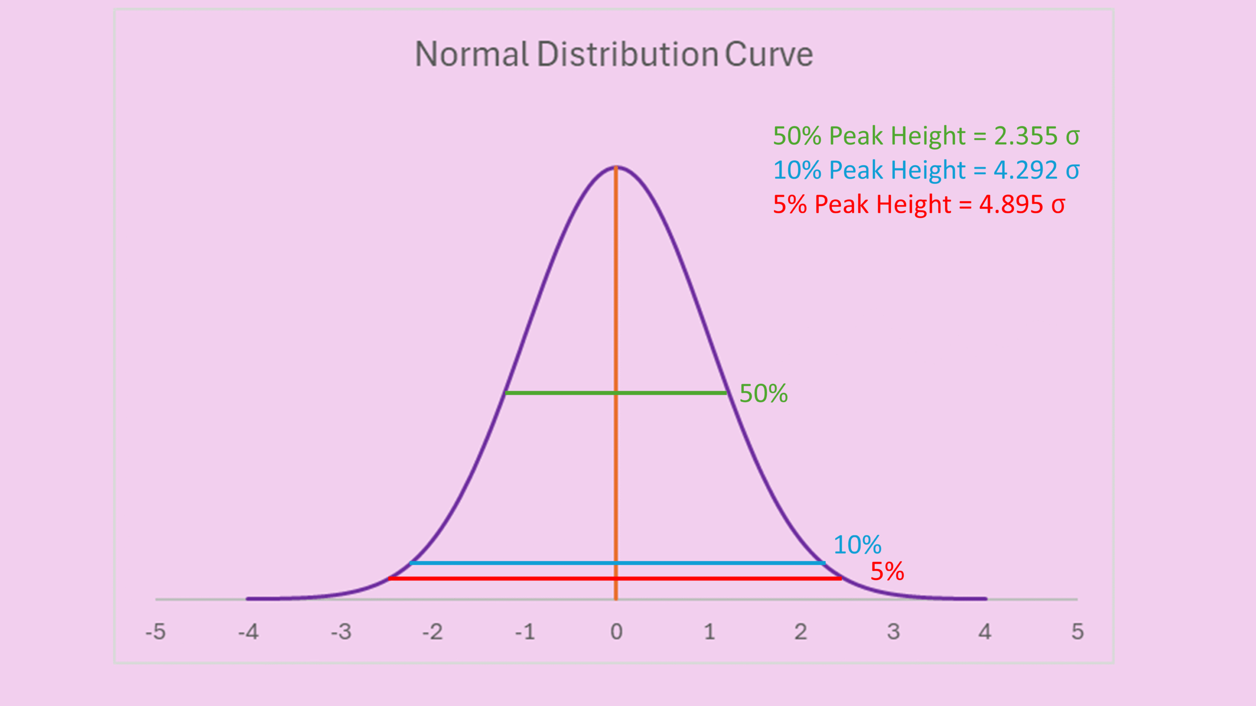
Peak width at half height (FWHM) can also be derived from Gaussian distribution formula.

\[ f(x)=\frac{1}{\sigma\sqrt{2\pi}} \; e^{-\frac{(x-\mu)^2}{2\sigma^2}} \] \[ \text{At } x=\mu,\quad f_{\max}=\frac{1}{\sigma\sqrt{2\pi}} \] \[ \text{At half height: } f(x)=\frac{1}{2}f_{\max} \] \[ \frac{1}{\sigma\sqrt{2\pi}} \; e^{-\frac{(x-\mu)^2}{2\sigma^2}} = \frac{1}{2} \cdot \frac{1}{\sigma\sqrt{2\pi}} \] \[ e^{-\frac{(x-\mu)^2}{2\sigma^2}} = \frac{1}{2} \] \[ -\frac{(x-\mu)^2}{2\sigma^2} = \ln\left(\frac{1}{2}\right) \] \[ (x-\mu)^2 = 2\sigma^2 \ln(2) \] \[ |x-\mu| = \sigma \sqrt{2\ln(2)} \] \[ \text{FWHM} = 2 \sigma \sqrt{2\ln(2)} \] \[ \text{FWHM}\approx 2.355\sigma \]

Similarly:

• 5% height → 4.895σ
• 10% height → 4.292σ

---

🔑 Key Takeaways

• Gaussian distribution chromatography explains both noise and peak behavior
• σ represents spread, not direct width
• 3σ and 4σ define practical peak boundaries
• Weighted calculations are required for peak analysis
• FWHM is directly linked to σ

---

🚀 Final Thoughts

Understanding this concept helps you move beyond treating peaks as black boxes. Instead, you start seeing the logic behind retention time, peak width, and detection limits.

If you’ve been working with GC for a while, this concept will connect many formulas you already use.

---

👉 What’s Next

In upcoming posts, I will show how Gaussian distribution chromatography connects to:

• Peak resolution
• Theoretical plates
• Those “mysterious constants” like 1.699 and 5.545